Products
Solutions
Resources
9977 N 90th Street, Suite 250 Scottsdale, AZ 85258 | 1-800-637-7496
© 2024 InEight, Inc. All Rights Reserved | Privacy Statement | Terms of Service | Cookie Policy | Do not sell/share my information

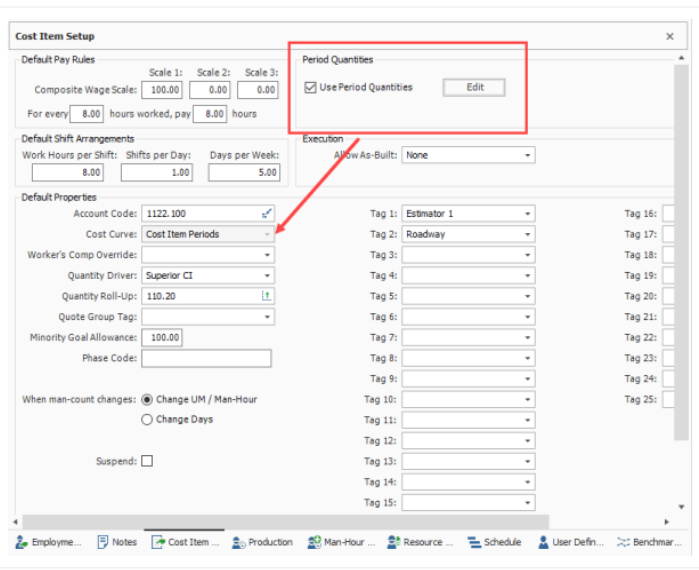
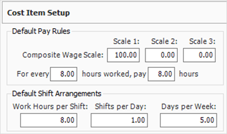
On the Cost Item Setup data block, you can adjust wage scale and shift arrangements for a specific cost item.
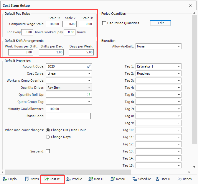
The composite wage scale and work and pay hours are used in the calculation of the cost of employed labor resources. The data reported on the Default Pay Rules tab is inherited from the composite wage scale and work and pay hours defined on the Job Properties > Cost Basis tab for the current job. These settings can be modified from the default on a cost item-by-cost item basis.
The Pay Rules for cost items can also be defined or modified on the Cost Breakdown Structure (CBS) Register in the Scale 1, Scale 2, Scale 3, Work Hours Rules, and/or Pay Hours Rules columns in the row of the subject cost item.
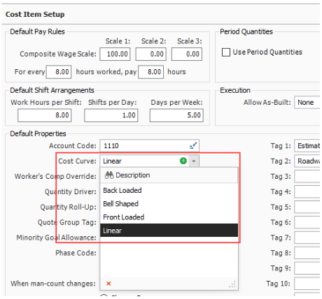
Cost curves are used to determine how the cost of a cost item is distributed over time. The main benefit of defining the cost curve for a cost item is to create a more accurate estimation of the cash flow over the life of a project.
The schedule dates entered on a cost item are used to define the periods across which a cost item incurs its costs. A cost item’s start and finish dates can be entered manually by the user or established using Schedule Integration, and the time periods (day, week, month, quarter, year) are determined in the Cash Flow settings in Job Properties. For more information about scheduling, see InEight Schedule integration.
By default, cost items have a linear cost curve, which distributes the cost equally across all periods for the cost item. There are 5 different types of cost curves that can be selected from the Cost Item Record > Cost Item Setup page.
| Cost curve type |
Definition |
|---|---|
|
Back Loaded |
Costs are low for most of an activity's timeline but then increase towards the end. This curve type starts out with a lower slope and gradually becomes steeper as the work progresses. Most resources are assumed to be consumed later in the activity and may be more characteristic of subcontracted work where costs are incurred as the work nears completion. |
| Bell Shaped | Expenses are low at the start of an activity, increase during construction, and decrease as the project approaches completion. Bell-shaped cost curves incur most of their costs towards the mid-point of the work and exponentially increase and decrease from the beginning to the end of the activity. This type of curve can be characteristic of larger portions of work that start with a few resources, ramp up to a peak, incurring more costs during the ramp up, then ramp back down as the work nears completion. |
| Front Loaded | A front-loaded cost curve is when costs are incurred early in an activity. This can happen for several reasons, such as early procurement of materials to take advantage of lower prices or to address long lead times. |
|
Linear |
Linear cost curves take the total cost of the activity and spreads it equally amongst the specified periods. |
|
Cost Item Periods |
Invoked by using the Period Quantities feature (described below). Cost Item Periods are used to customize cost curves based on the quantities consumed in various periods. In comparison to the other curves which spread the items total cost proportionally based the chosen cost curve, the Cost Item Periods option can generate a more precise distribution of costs to specific periods because the user can simply define how much quantity of work is getting completed in each specific period.
|
You can also choose to create your own custom cost curve by clicking the Add button in the Cost Curve drop-down menu.
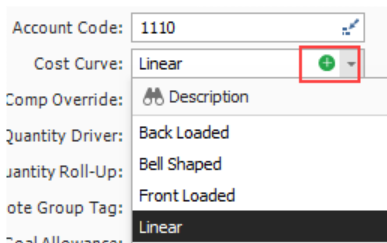
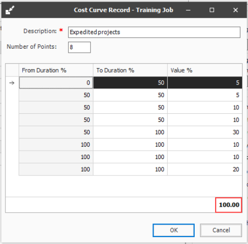
Custom cost curves let you define your own from and to durations along with their associated values, which need to add up to 100%.
All cost curves, regardless of type, impact the generation of the cash flow graph. The Cash Flow form provides a graphical representation of the cash flow and resource utilization of your project. For more information, see Cash flow overview.
The Cash Flow options are used to define the cash flow rules (revenue timing, cost timing, cost of money, and quantities) needed to calculate the finance expense and cash flow for your project. For more information, see Cash flow options.
You can control what information shows on the Cash Flow graph in the cash flow display settings. For more information, see Cash flow display settings.
Like the other four cost curves, Period Quantities are used to customize cost curves, which show you a graphical representation of the cash flow and resource utilization so you can assess the proper financing and resource project needs. When the Period Quantities check box is selected, the Cost Curve automatically changes to Cost Item Periods.
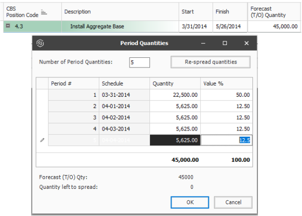
The Period Quantity calculator uses the cost item quantity assigned to various periods to calculate the specific percentages attributable to each range of periods covered by the cost item. The purpose of using period quantities is to spread costs via the cost curve in the cash flow analysis. For example, if you have an item where 50% of the cost is incurred when you start the work because you have to buy all the material first, then you would want a customized cost curve to reflect that this is how the costs will be incurred over time when building that work.
In the example below, since 50% of the cost is incurred when the project starts, period one's quantity is 50% of 45,000 Forecast (T/O) Qty, which is 22,500. The remaining costs are then spread equally across the remaining three periods.
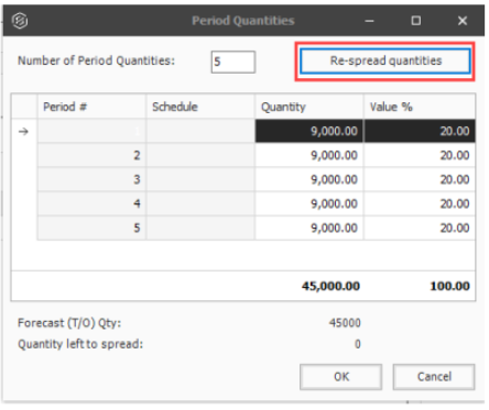
You can also choose to select the Re-spread quantities button to spread the quantities equally among the periods entered in the Number of Period Quantities field.
From the Estimate tab, select Cost Breakdown Structure (CBS).
Right-click the row header for a cost item and select Open.
Select the Cost Item Setup tab in the lower-right portion of the form (the tab name may be abbreviated).
In the Default Pay Rules data block, adjust your Composite Wage Scale as needed.
Under the Composite Wage Scale, adjust the number of hours and paid as needed
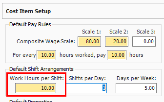
In the Default Shift Arrangements data block, make changes as needed.
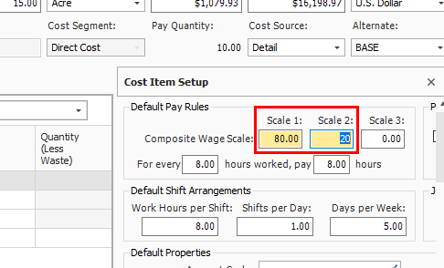
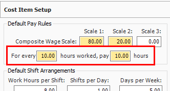
For this example, we’ll make the following changes on the Clearing cost item:
Composite Wage Scale – 80% Scale 1, 20% Scale 2.
For every 10 hours worked, pay 10 hours.
Default Shift Arrangements – Change Work Hours per Shift to 10.
Additional Information
9977 N 90th Street, Suite 250 Scottsdale, AZ 85258 | 1-800-637-7496
© 2024 InEight, Inc. All Rights Reserved | Privacy Statement | Terms of Service | Cookie Policy | Do not sell/share my information